


There are different parts of Data Visualization
• Analyze Numbers: Analyze numbers by different ways. We’ll do different types of calculations on
numbers and understand how we can do them.
• Visualize the data through Data Visualization: We can make lot of Graphs of different type to
understand about different things. We can make graphs to understand how many marks you have
scored and other things.
But how we will analyse the data we need tools right. So we have got different python libraries to do the
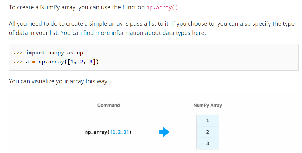
There is one such library called as Numpy. Do you remember the List which we did when we were
learning Python. It is very much same to that.In Numpy we call it Array.
| Python List | NumPy Array |
| Be Able to store different data types in the e same list | Can store only one data type in an array at anytime |
| The reason because it have different data e it is not so fast. | The data is stored at the same sequence so types they are saved at different places so itis faster. |
Numpy
NumPy (Numerical Python) is an open source Python library that’s used in almost every field of science and engineering. It’s the universal standard for working with numerical data in Python, and it’s at the core of the scientific Python Data manipulation in Python is nearly synonymous with NumPy array manipulation: even newer tools like Pandas are built around the NumPy array. This section will present several examples of using NumPy array manipulation to access data and subarrays, and to split, reshape, and join the arrays. While the types of operations shown here may seem a bit dry and rule based, they comprise the building blocks of many other examples.
Get to know them well!
We’ll cover a few categories of basic array manipulations here:
- Attributes of arrays: Determining the size, shape, memory consumption, and data types of arrays
- Indexing of arrays: Getting and setting the value of individual array elements
- Slicing of arrays: Getting and setting smaller subarrays within a larger array
- Reshaping of arrays: Changing the shape of a given array
- Joining and splitting of arrays: Combining multiple arrays into one, and splitting one array into many
NumPy Array Attributes
First let’s discuss some useful array attributes. We’ll start by defining three random arrays, a one-dimensional, two-dimensional, and three-dimensional array. We’ll use NumPy’s random number generator, which we will seed with a set value in order to ensure that the same random arrays are generated each time this code is run:

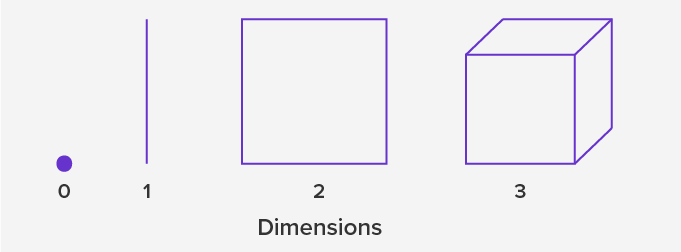
The teacher needs to discuss the one dimension, two dimensions and three dimensions. It’s like writing in one line or having just length. Then writing on two dimensions is like writing on length and breadth both and then writing on three dimensions is like length, breadth and height so it can be explained like there is a line, square and then cube.
[ ]
import numpy as np # This is how we import the numpy.

x1 = np.random.randint(1,10, size=6)  # One-dimensional array
x2 = np.random.randint(1,10, size=(3, 4))  # Two-dimensional array. It tells that 3 rows and 3 columns need to be there.
x3 = np.random.randint(1,10, size=(3, 4, 5))  # Three-dimensional array. It tells 3 tables will be generated with 4 rows and 5 columns. Take time and explain.
print(x1)
print()
print(x2)
print()
print(x3)
# As many time you click on above play button a random number will be generated.
# Explain that numbers in just one square bracket are like one dimension, then two and three accordingly.
We have generated x1,x2 and x3 to use it’s value throughout the session.
Each array has attributes ndim (the number of dimensions), shape (the size of each dimension), and size (the total size of the array):
print("x3 ndim: ", x3.ndim)
print("x3 shape:", x3.shape)
print("x3 size: ", x3.size)
x3 ndim:  3
x3 shape: (3, 4, 5)
x3 size:  60
Find the dimension, shape and size of x2 and x1.


The synatx is ‘arange’ not arrange. Single r is there.

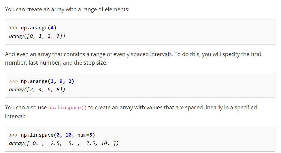
# Made to do the above three condtions.
# Explain the difference between the above three codes and ask if the  can write multiplication table of any number using arange() and linspace

print(np.arange(6,60,6)) # Just like the for loop the final condition in arange i.e. 60 here is not considred.

print(np.linspace(0,180,num=10))
[ 6 12 18 24 30 36 42 48 54]
[  0.  20.  40.  60.  80. 100. 120. 140. 160. 180.]
Array Indexing: Accessing Single Elements
Don’t forget to about the index starts with 0. So the index of first row will be zero and column will be zero too.
If you are familiar with Python’s standard list indexing, indexing in NumPy will feel quite familiar. In a one-dimensional array, the ith value (counting from zero) can be accessed by specifying the desired index in square brackets, just as with Python lists:
x1
array([9, 3, 5, 3, 4, 4])
x1[0]
9
x1[4]
4
To index from the end of the array, you can use negative indices:
x1[-1]
4
x1[-2]
4
In a multi-dimensional array, items can be accessed using a comma-separated tuple of indices:
x2
array([[1, 4, 5, 8],
       [4, 1, 6, 9],
       [5, 4, 2, 8]])
x2[0, 0]
1
x2[2, 0]
5
x2[2, -1]
8
Values can also be modified using any of the above index notation:
[
x2[0, 0] = 12
x2
array([[12,  4,  5,  8],
       [ 4,  1,  6,  9],
       [ 5,  4,  2,  8]])
Keep in mind that, unlike Python lists, NumPy arrays have a fixed type. This means, for example, that if you attempt to insert a floating-point value to an integer array, the value will be silently truncated. Don’t be caught unaware by this behavior! Truncated means 15.2 will become 15.
x1[0] = 3.14159  # this will be truncated!
x1
array([3, 3, 5, 3, 4, 4])
Array Slicing: Accessing Subarrays
Just as we can use square brackets to access individual array elements, we can also use them to access subarrays with the slice notation, marked by the colon (:) character. The NumPy slicing syntax follows that of the standard Python list; to access a slice of an array x, use this:
x[start:stop:step]If any of these are unspecified, they default to the values start=0, stop=size of dimension, step=1. We’ll take a look at accessing sub-arrays in one dimension and in multiple dimensions.
One-dimensional subarrays
[ ]
x = np.arange(10)
x
array([0, 1, 2, 3, 4, 5, 6, 7, 8, 9])
[ ]
x[:5] # first five elements
array([0, 1, 2, 3, 4])
[ ]
x[5:] # elements after index 5
array([5, 6, 7, 8, 9])
[ ]
x[4:7] # middle sub-array
array([4, 5, 6])
[ ]
x[::2] # every other element
array([0, 2, 4, 6, 8])
[ ]
x[1::2] # every other element, starting at index 1
array([1, 3, 5, 7, 9])
A potentially confusing case is when the step value is negative. In this case, the defaults for start and stop are swapped. This becomes a convenient way to reverse an array:
[ ]
x[::-1] # all elements, reversed
array([9, 8, 7, 6, 5, 4, 3, 2, 1, 0])
[ ]
x[5::-2] # reversed every other from index 5
array([5, 3, 1])


