


We learnt a lot about the Numpy it’s basic introduction and all what we can do with it. Now we’ll get more into it and learn few more syntax of numpy. We were learning how to access one-dimensional subarray and do slicing operations on it. Now we’ll see for multidimensional.
The below cell is getting repeated to have proper arrays of all three dimensions to work on.
import numpy as np # This is how we import the numpy.

x1 = np.random.randint(1,10, size=6)  # One-dimensional array
x2 = np.random.randint(1,10, size=(9, 9))  # Two-dimensional array. It tells that 9 rows and 9 columns need to be there.
x3 = np.random.randint(1,10, size=(6, 3, 3))  # Three-dimensional array. It tells 6 tables will be generated with 3 rows and 3 columns
print(x1)
print()
print(x2)
print()
print(x3)
# As many time you click on above play button a random number will be generated.
[3 8 2 5 3 4]

[[4 8 6 4 3 2 9 7 7]
 [4 4 7 8 3 4 9 4 8]
 [6 4 6 4 2 9 7 2 3]
 [5 7 7 7 1 5 6 1 2]
 [7 7 1 3 3 9 7 5 8]
 [6 1 9 7 1 7 2 5 6]
 [8 7 1 8 8 8 3 1 9]
 [2 6 1 2 4 6 7 6 9]
 [6 2 9 9 4 5 3 8 4]]

[[[9 6 6]
  [5 7 9]
  [1 1 1]]

 [[4 2 1]
  [6 4 3]
  [6 7 5]]

 [[8 2 7]
  [5 5 9]
  [6 1 8]]

 [[6 2 7]
  [3 9 8]
  [1 4 4]]

 [[7 5 5]
  [8 2 7]
  [3 1 7]]

 [[9 3 6]
  [4 1 9]
  [9 4 5]]]
Multi-dimensional subarrays
Multi-dimensional slices work in the same way, with multiple slices separated by commas. For example:
x2 #The x2's value is coming from the top cell which we created using random function.
array([[4, 8, 6, 4, 3, 2, 9, 7, 7],
       [4, 4, 7, 8, 3, 4, 9, 4, 8],
       [6, 4, 6, 4, 2, 9, 7, 2, 3],
       [5, 7, 7, 7, 1, 5, 6, 1, 2],
       [7, 7, 1, 3, 3, 9, 7, 5, 8],
       [6, 1, 9, 7, 1, 7, 2, 5, 6],
       [8, 7, 1, 8, 8, 8, 3, 1, 9],
       [2, 6, 1, 2, 4, 6, 7, 6, 9],
       [6, 2, 9, 9, 4, 5, 3, 8, 4]])
x2[:2, :3] # two rows, three columns
array([[4, 8, 6],
       [4, 4, 7]])
x2[:3, ::2] # all rows, every other column
array([[4, 6, 3, 9, 7],
       [4, 7, 3, 9, 8],
       [6, 6, 2, 7, 3]])
Finally, subarray dimensions can even be reversed together:
x2[::-1,::-1]
array([[4, 8, 3, 5, 4, 9, 9, 2, 6],
       [9, 6, 7, 6, 4, 2, 1, 6, 2],
       [9, 1, 3, 8, 8, 8, 1, 7, 8],
       [6, 5, 2, 7, 1, 7, 9, 1, 6],
       [8, 5, 7, 9, 3, 3, 1, 7, 7],
       [2, 1, 6, 5, 1, 7, 7, 7, 5],
       [3, 2, 7, 9, 2, 4, 6, 4, 6],
       [8, 4, 9, 4, 3, 8, 7, 4, 4],
       [7, 7, 9, 2, 3, 4, 6, 8, 4]])
Accessing array rows and columns
One commonly needed routine is accessing of single rows or columns of an array. This can be done by combining indexing and slicing, using an empty slice marked by a single colon (:) :
print(x2[:, 0]) # first column of x2
[4 4 6 5 7 6 8 2 6]
print(x2[0, :]) # first row of x2
[4 8 6 4 3 2 9 7 7]
In the case of row access, the empty slice can be omitted for a more compact syntax:
print(x2[0]) # equivalent to x2[0, :]
[4 8 6 4 3 2 9 7 7]
Subarrays without copying and changing in real values.
One important–and extremely useful–thing to know about array slices is that they return views rather than copies of the array data. This is one area in which NumPy array slicing differs from Python list slicing: in lists, slices will be copies. That means whatever change we’ll make in NumPy array it will be permanent. Consider our two-dimensional array from before:
print(x2)
[[4 8 6 4 3 2 9 7 7]
 [4 4 7 8 3 4 9 4 8]
 [6 4 6 4 2 9 7 2 3]
 [5 7 7 7 1 5 6 1 2]
 [7 7 1 3 3 9 7 5 8]
 [6 1 9 7 1 7 2 5 6]
 [8 7 1 8 8 8 3 1 9]
 [2 6 1 2 4 6 7 6 9]
 [6 2 9 9 4 5 3 8 4]]
Let’s extract a 2×2 subarray from this:
x2_sub = x2[:2, :2]

print(x2_sub)
[[4 8]
 [4 4]]
Now if we modify this subarray, we’ll see that the original array is changed! Observe:
x2_sub[0, 0] = 99

print(x2_sub)
[[99  8]
 [ 4  4]]
print(x2)
[[99  8  6  4  3  2  9  7  7]
 [ 4  4  7  8  3  4  9  4  8]
 [ 6  4  6  4  2  9  7  2  3]
 [ 5  7  7  7  1  5  6  1  2]
 [ 7  7  1  3  3  9  7  5  8]
 [ 6  1  9  7  1  7  2  5  6]
 [ 8  7  1  8  8  8  3  1  9]
 [ 2  6  1  2  4  6  7  6  9]
 [ 6  2  9  9  4  5  3  8  4]]
This default behavior is actually quite useful: it means that when we work with large datasets, we can access and process pieces of these datasets without the need to copy the underlying data buffer.
Creating copies of arrays
Despite the nice features of array views, it is sometimes useful to instead explicitly copy the data within an array or a subarray. This can be most easily done with the copy() method:
x2_sub_copy = x2[:2, :2].copy()
print(x2_sub_copy)
[[99  8]
 [ 4  4]]
If we now modify this subarray, the original array is not touched:
x2_sub_copy[0, 0] = 42

print(x2_sub_copy)
[[42  8]
 [ 4  4]]
print(x2)
[[99  8  6  4  3  2  9  7  7]
 [ 4  4  7  8  3  4  9  4  8]
 [ 6  4  6  4  2  9  7  2  3]
 [ 5  7  7  7  1  5  6  1  2]
 [ 7  7  1  3  3  9  7  5  8]
 [ 6  1  9  7  1  7  2  5  6]
 [ 8  7  1  8  8  8  3  1  9]
 [ 2  6  1  2  4  6  7  6  9]
 [ 6  2  9  9  4  5  3  8  4]]
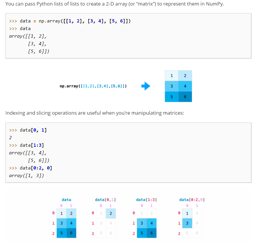
In the below picture we can see how to make 2D Array without using any function. Earlier we were putting the values through random function now we will put in ourselves.

Problem Statement: Let’s say there are people standing in particular way in rows and columns and we want people to swap that means people standing in rows make columns and other way round too.
That’s called transpose.

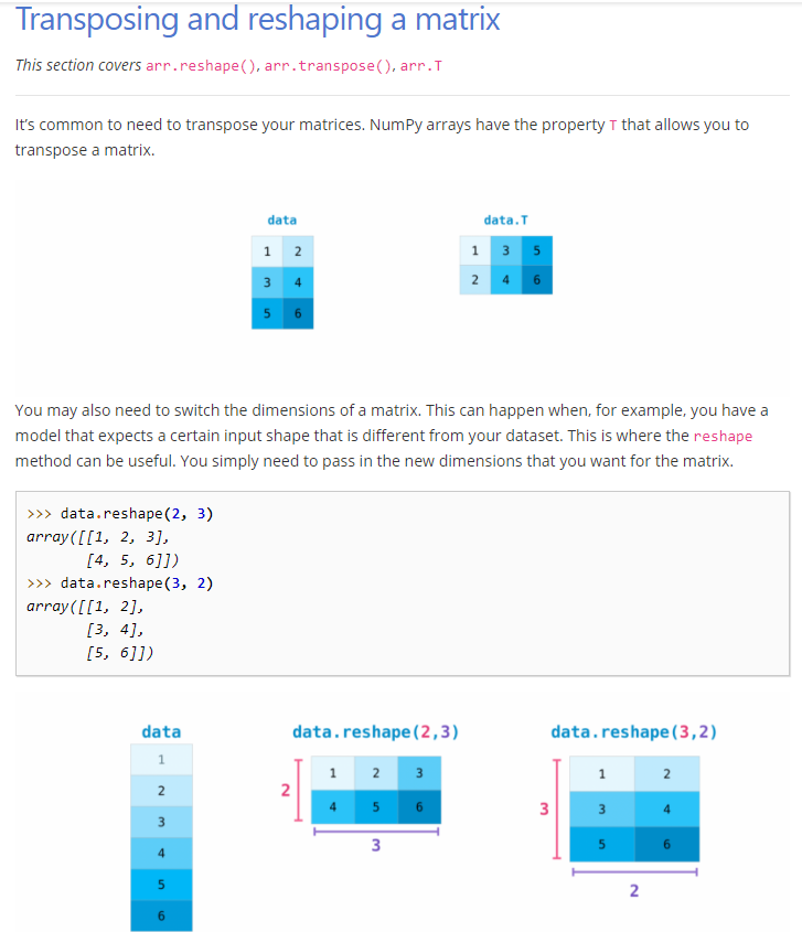

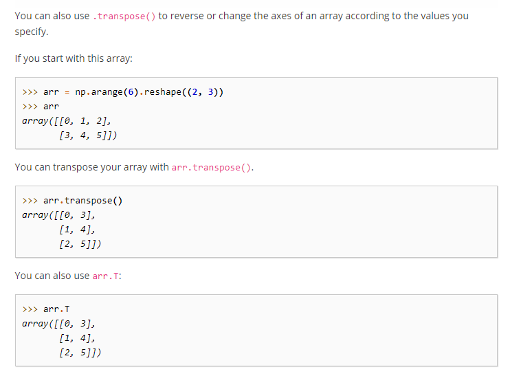
Reshaping of Arrays
Another useful type of operation is reshaping of arrays. The most flexible way of doing this is with the reshape method. For example, if you want to put the numbers 1 through 9 in a 3×3 grid, you can do the following:
grid = np.arange(1, 10).reshape((3, 3))
print(grid)
[[1 2 3]
 [4 5 6]
 [7 8 9]]
Note that for this to work, the size of the initial array must match the size of the reshaped array. Where possible, the reshape method will use a no-copy view of the initial array, but with non-contiguous memory buffers this is not always the case.
Another common reshaping pattern is the conversion of a one-dimensional array into a two-dimensional row or column matrix. This can be done with the reshape method, or more easily done by making use of the newaxis keyword within a slice operation:
x = np.array([1, 2, 3])

# row vector via reshape
x.reshape((1, 3))
array([[1, 2, 3]])
# row vector via newaxis
x[np.newaxis, :]
array([[1, 2, 3]])
# column vector via reshape
x.reshape((3, 1))
array([[1],
       [2],
       [3]])
# column vector via newaxis
x[:, np.newaxis]
array([[1],
       [2],
       [3]])
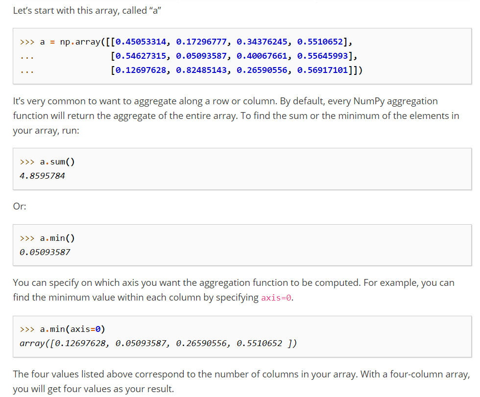
Make an array and find sum, max and min in it.


